Paul Campos reminds us that this discussion Detroit Pro Basketball Team Records:
The Detroit Pistons lost 27 games in a row last night, breaking the NBA record for most consecutive losses in a season. . . . A team's record, broadly speaking, is a function of two factors.
(1) Team quality. „Quality“ means anything about a team's performance that is not the result of chance factors, aka luck. Players' individual and collective abilities, quality of coaching, quality of team management, e.g.
(2) Random element, aka luck.
Are luck and skill relatively important?
The post linked above continues as follows:
How do we disentangle the relative importance of these two factors when evaluating a team's performance up to a point in the season? . . The best predictor of a team's performance in advance is the ratings of those betting on its performance. Although I recognize that gambling odds can sometimes contain significant inefficiencies in the form of the public making emotional bets rather than calmly rational bets, this is the exception rather than the rule. . . . Detroit's final even money over/under for winning percentage this season was .340 winning percentage before the first game was played. A little more than a third of the way through the season, Detroit's winning percentage is .0666. . . .
To the extent that the team suffered from unusual bad luck, one would expect the team's final performance to be much better. But how good is it? Here we can once again turn to the pundits of Las Vegas et al. He is currently setting even odds for the team's final record based on the assumption that the winning percentage for remaining games is .170.
Campos shared his purported Bayesian analysis and summarized it as follows: “Given just two pieces of information, the up-front assumption of a .340 team and the subsequent information of a .066 performance over 30 games, when you combine those two pieces of information, you get: ” The prediction is that the future winning probability will be 0.170, which surprisingly is exactly what the current gambling odds are predicting. . . . Estimates made by professional gamblers suggest that about two-thirds of Detroit's worse-than-expected performance is the result of overestimating the quality of the team in advance, and the remaining one-third is due to bad luck. It seems that it is considered. ”
I think the last statement comes from the fact that (1/3)*0.340 + (2/3)*0.067 is approximately 0.170.
I don't really follow his Bayesian logic. But don't worry about it for now.
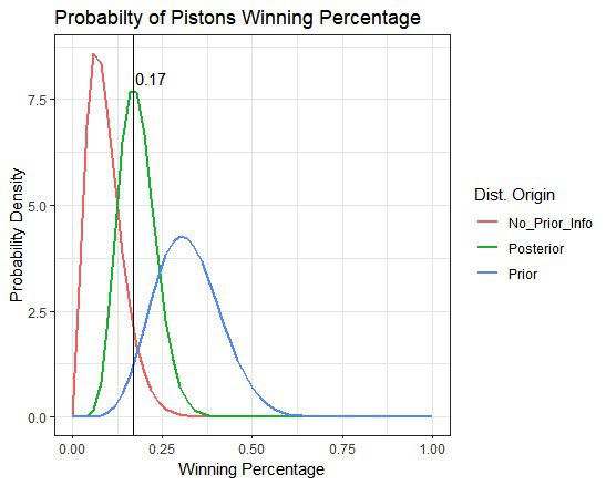
As I said earlier, I did not fully subscribe to the Bayesian logic shared by Mr. Campos. Here's my problem. He posted the following graph.

I think I understand the „No_Prior_Info“ curve in the graph. This is the likelihood of y ~ binomial(n, p) for p with data n=30 and y=2. But I don't understand where the „prior“ and „posterior“ curves come from. I believe the mean of the prior distribution is 0.340 and the mean of the posterior distribution is 0.170, but where do the widths of these curves come from?
Part of the confusion here is that we're dealing with inferring p (the „quality“ of a team summarized by the probability of winning against a randomly chosen opponent on a random day) and predicting the outcome. Regarding the posterior mean, there is no difference. In the basic model, the posterior expected proportion of future game wins is equal to the posterior mean of p. Talking about uncertainty on the page makes it even more difficult.
So how can we make sense of the betting lines at the beginning of the season and now? For the purposes of this discussion, we will identify this as a back and forth betting line. means Values of p and implicit ex-ante and ex-post excerpts ignoring bettors' systematic biases. distribution?We're sure there's enough information here to do this, using input from all 30 teams and adjusting appropriately.?
Exploratory analysis
I started by going online, finding various sources of information on betting odds, team records, and goal differentials, and entering the data. this file. The most recent Las Vegas odds I could find in the season record were for him on December 19th. All other data are from December 27th.
The next step was to create some graphs. First, we looked at the goal difference and team performance so far.
nbaHere's a question you should always ask yourself: What do you expect to see?
Before performing any statistical analysis it's good practice to anticipate the results. So what do you think these graphs will look like?
- Ppg scored vs. ppg allowed. What do you expect to see? Before making the graph, I could have imagined it going either way: you might expect a negative correlation, with some teams doing the run-and-gun and others the physical game, or you might expect a positive correlation, because some teams are just much better than others. My impression is that team styles don't vary as much as they used to, so I was guessing a positive correlation.
- Won/lost record vs. point differential. What do you expect to see? Before making the graph, I was expecting a high correlation. Indeed, if I could only use one of these two metrics to estimate a team's ability, I'd be inclined to use point differential.Aaaand, here's what we found:
Hey, my intuition worked on these! It would be interesting to see data from other years to see if I just got lucky with that first one.
Which is a better predictor of won-loss record: ppg scored or ppg allowed?
OK, this is a slight distraction from Campos's question, but now I'm wondering, which is a better predictor of won-loss record: ppg scored or ppg allowed? From basic principles I'm guessing they're about equally good.
Let's do a couple of graphs:
pdf("nba2023_2.pdf", height=3.5, width=10) par(mfrow=c(1,3), oma=c(0,0,2,0)) par(mar=c(3,3,1,1), mgp=c(1.5,.5,0), tck=-.01) # par(pty="m") rngWhich yields:
So, about what we expected. To round it out, let's try some regressions:
library("rstanarm") print(stan_glm(record ~ ppg, data=nba, refresh=0), digits=3) print(stan_glm(record ~ ppg_a, data=nba, refresh=0), digits=3) print(stan_glm(record ~ ppg + ppg_a, data=nba, refresh=0), digits=3)result:
Median MAD_SD (Intercept) -1.848 0.727 ppg 0.020 0.006 Auxiliary parameter(s): Median MAD_SD sigma 0.162 0.021 ------ Median MAD_SD (Intercept) 3.192 0.597 ppg_a -0.023 0.005 Auxiliary parameter(s): Median MAD_SD sigma 0.146 0.019 ------ Median MAD_SD (Intercept) 0.691 0.335 ppg 0.029 0.002 ppg_a -0.030 0.002 Auxiliary parameter(s): Median MAD_SD sigma 0.061 0.008In other words, goals scored and goals conceded are roughly equal predictors of win-loss record. Considering that, it makes sense to recode as ppg difference points and total points.
print(stan_glm(record ~ ppg_diff + I(ppg + ppg_a), data=nba, refresh=0), digits=3)Here's what you get:
Median MAD_SD (Intercept) 0.695 0.346 ppg_diff 0.029 0.002 I(ppg + ppg_a) -0.001 0.001 Auxiliary parameter(s): Median MAD_SD sigma 0.062 0.009check. If you include ppg_diff as a predictor, the average total points will be of little use. Again, 30 games for each team doesn't provide much of a sample, so it's best to look at data from other seasons.
Now to the betting line
Now let's include the Las Vegas over-under in our analysis. First, here are some graphs.
pdf("nba2023_3.pdf", height=3.5, width=10) par(mfrow=c(1,3), oma=c(0,0,2,0)) par(mar=c(3,3,1,1), mgp=c(1.5,.5,0), tck=-.01) # par(pty="s") rngWhich yields:
Oops--I forgot to make some predictions before looking. In any case, the first graph is kinda surprising. You'd expect to see an approximate pattern of E(y|x) = x, and we do see that--but not at the low end. The teams that were predicted to do the worst this year are doing even worse than expected. It would be interesting to see the corresponding graph for earlier years. My guess is that this year is special, not only in the worst teams doing so bad, but in them underperforming their low expectations.
The second graph is as one might anticipate: Betters are predicting some regression toward the mean. Not much, though! And the third graph doesn't tell us much beyond the first graph.
Upon reflection, I'm finding the second graph difficult to interpret. The trouble is that "Betting line in Dec" is the forecast win percentage for the year, but 30/82 of that is the existing win percentage. (OK, not every team has played exactly 30 games, but close enough.) What I want to do is just look at the forecast for their win percentage for the rest of the season:
pdf("nba2023_4.pdf", height=3.5, width=10) par(mfrow=c(1,3), oma=c(0,0,2,0)) par(mar=c(3,3,1,1), mgp=c(1.5,.5,0), tck=-.01) # par(pty="s") rngHere's the graph:
The fitted regression line has a slope of 0.66:
Median MAD_SD (Intercept) 0.17 0.03 record 0.66 0.05 Auxiliary parameter(s): Median MAD_SD sigma 0.05 0.01The next step is to predict Las Vegas' projections for the rest of the season, taking into account the initial predictions and the team's record thus far.
print(stan_glm(future_odds ~ start_odds + record, data=nba, refresh=0), digits=2) Median MAD_SD (Intercept) -0.02 0.03 start_odds 0.66 0.10 record 0.37 0.06 Auxiliary parameter(s): Median MAD_SD sigma 0.03 0.00The funny thing is, everywhere I look I see this 0.66. And his 30 games equals 37% of his season.
Now let's add the points per game difference to the regression analysis. This should include additional information beyond that contained in previous wins and losses.
print(stan_glm(future_odds ~ start_odds + record + ppg_diff, data=nba, refresh=0), digits=2) Median MAD_SD (Intercept) 0.06 0.06 start_odds 0.67 0.09 record 0.20 0.11 ppg_diff 0.01 0.00 Auxiliary parameter(s): Median MAD_SD sigma 0.03 0.00ppg_diff is different from other scales, so this is difficult to interpret. Let's quickly standardize it to the same scale as our previous win/loss records.
nba$ppg_diff_stdOK, not enough data to cleanly disentangle won-lost record and point differential as predictors here. My intuition would be that, once you have point differential, the won-lost record tells you very little about what will happen in the future, and the above fitted model is consistent with that intuition, but it's also consistent with the two predictors being equally important, indeed it's consistent with point differential being irrelevant conditional on won-lost record.
What we'd want to do here--and I know I'm repeating myself--is to repeat the analysis using data from previous years.
Interpreting the implied Vegas prediction for the rest of the season as an approximate weighted average of the preseason prediction and the current won-lost record
In any case, the weighting seems clear: approx two-thirds from starting odds and one-third from the record so far, which at least on a naive level seems reasonable, given that the season is about one-third over.
Just for laffs, we can also throw in difficulty of schedule, as that could alter our interpretation of the teams' records so far.
nba$sched_stdSo, strength of schedule does not supply much information. This makes sense, given that 30 games is enough for the teams' schedules to mostly average out.
The residuals
Now that I've fit the regression, I'm curious about the residuals. Let's look:
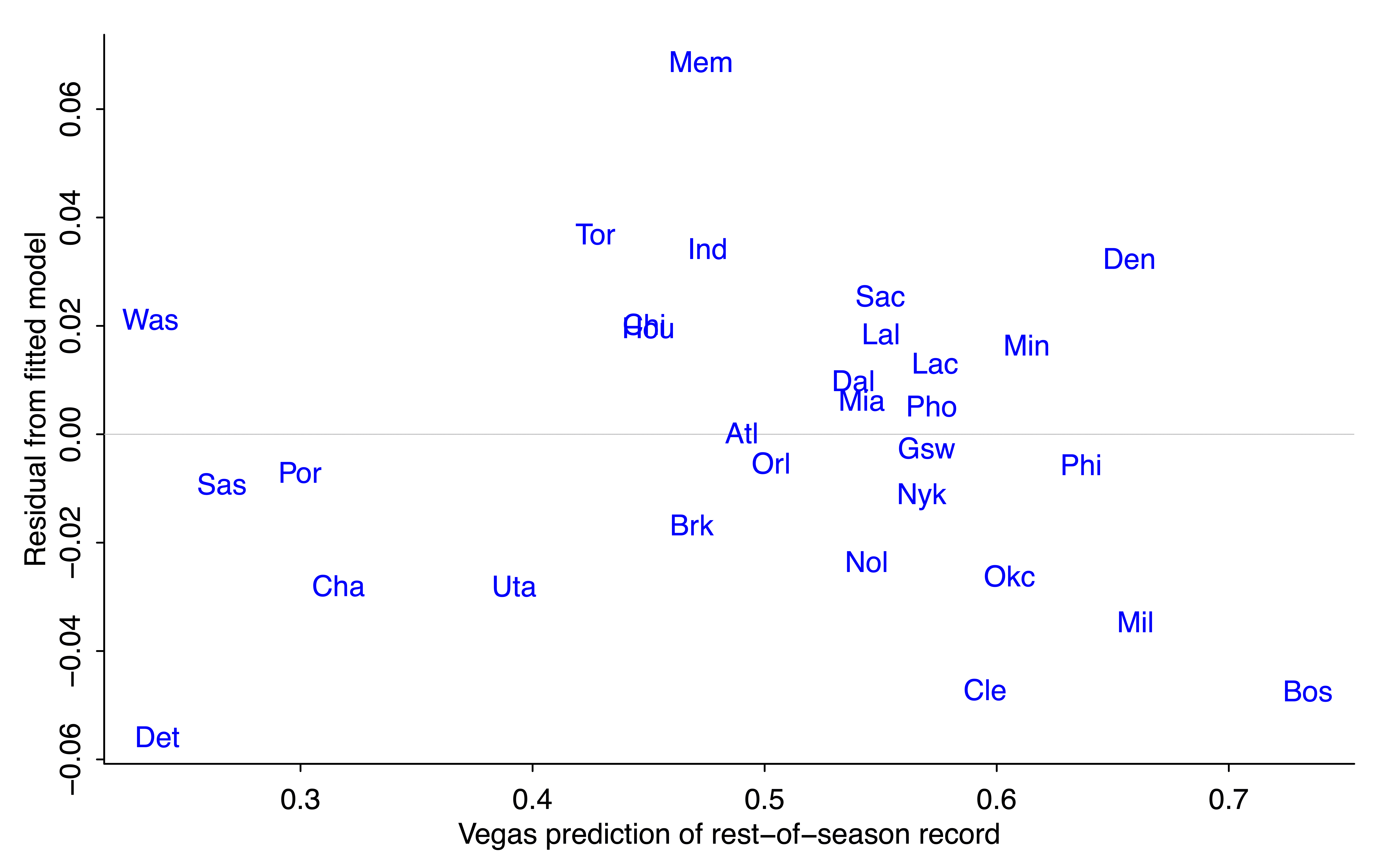
fit_5And here's the graph:
The residual for Detroit is negative (-0.05*52 = -2.6, so the Pistons are expected to win about 3 games less than their regression prediction based on prior odds and outcome of first 30 games). Cleveland and Boston are also expected to do a bit worse than the model would predict. On the other direction, Vegas is predicting that Memphis will win about 4 games more than predicted from the regression model.
I have no idea whassup with Memphis. The quick generic answer is that the regression model is crude, and bettors have other information not included in the regression.
Reverse engineering an implicit Bayesian prior
OK, now for the Bayesian analysis. As noted above, we aren't given a prior for team j's average win probability, p_j; we're just given a prior point estimate of each p_j.
But we can use the empirical prior-to-posterior transformation, along with the known likelihood function, under the simplifying assumption the 30 win-loss outcomes for each team j are independent with constant probability p_j for team j. This assumption that is obviously wrong, given that teams are playing each other, but let's just go with it here, recognizing that with full data it would be straightforward to extend to an item-response model with an ability parameter for each team (as here).
To continue, the above regression models show that the Vegas "posterior Bayesian" prediction of p_j after 30 games is approximately a weighted average of 0.65*(prior prediction) + 0.35*(data won-loss record). From basic Bayesian algebra (see, for example, chapter 2 of BDA), this tells us that the prior has about 65/35 as much information as data from 30 games. So, informationally, the prior is equivalent to the information from (65/35)*30 = 56 games, about two-thirds of a season worth of information.
Hey--what happened??
But, wait! That approximate 2/3 weighting for the prior and 1/3 weighting of the data from 30 games is the opposite of what Campos reported, which was a 1/3 weighting of the prior and 2/3 of the data. Recall: prior estimated win probability of 0.340, data win rate of 0.067, take (1/3)*0.340 + (2/3)*0.067 and you get 0.158, which isn't far from the implied posterior estimate of 0.170.
What happened here is that the Pistons are an unusual case, partly because the Vegas over-under for their season win record is a few percentage points lower than the linear model predicted, and partly because when the probability is low, a small percentage-point change in the probability corresponds to a big change in the implicit weights.
Again, it would be good to check all this with data from other years.
Skill and luck
There's one more loose end, and that's Campos taking the weights assigned to data and prior and characterizing them as "skill" and "luck" in prediction errors. I didn't follow that part of the reasoning at all so I'll just let it go for now. Part of the problem here is in one place Campos seems to be talking about skill and luck as contributors to the team's record, and in another place he seems to considering them as contributors to the difference between preseason predictions and actual outcomes.
One way to think about skill and luck in a way that makes sense to me is within an item-response-style model in which the game outcome is a stochastic function of team abilities and predictable factors. For example, in the model,
score differential = ability of home team - ability of away team + home-field advantage + error,
the team abilities are in the "skill" category and the error is in the "luck" category, and, ummm, I guess home-field advantage counts as "skill" too? OK, it's not so clear that the error in the model should all be called "luck." If a team plays better against a specific opponent by devising a specific offensive/defensive plan, that's skill, but it would pop up in the error term above.
In any case, once we've defined what is skill and what is luck, we can partition the variance of the total to assign percentages to each.
Another way of looking at this is to consider the extreme case of pure luck. If outcomes determined only by luck, then each game is a coin flip, and we'd see this in the data because the team win proportions after 30 games would follow a binomial distribution with n=30 and p=0.5. The actual team win proportions have mean 0.5 (of course) and sd 0.18, as compared to the theoretical mean of 0.5 and sd of 0.5/sqrt(30) = 0.09. That simple calculation suggests that skill is (0.18/0.09)^2 = 4 times as important as luck when determining the outcome of 30 games.
And maybe I'm getting just getting this all tangled myself. The first shot at any statistical analysis often will have some mix of errors in data, modeling, computing, and general understanding, with that last bit corresponding to the challenge of mapping from substantive concepts to mathematical and statistical models. Some mixture of skill and luck, I guess.
Summary
1. Data are king. In the immortal words of Hal Stern, the most important aspect of a statistical analysis is not what you do with the data, it’s what data you use. I could do more than Campos did, not so much because of my knowledge of Bayesian statistics but because I was using data from all 30 teams.
2. To continue with that point, you can do lots better than me by including data from other years.
3. Transparency is good. All my data and code are above. I might well have made some mistakes in my analyses, and, in any case, many loose ends remain.
4. Basketball isn't so important (hot hand aside). The idea of backing out an effective prior by looking at information updating, that's a more general idea worth studying further. This little example is a good entry point into the potential challenge of such studies.
5. Models can be useful, not just for prediction but also for understanding, as we saw for the problem of partitioning outcomes into skill and luck.
P.S. Last week, when the Pistons were 2-25 or something like that, I was taking with someone who's a big sports fan but not into analytics, the kind of person who Bill James talked about when he said that people interpret statistics as words that describe a situation rather than as numbers that can be added, subtracted, multiplied, and divided. The person I was talking with predicted that the Pistons would win no more than 6 games this year. I gave the statistical argument why this was unlikely: (a) historically there's been regression to the mean, with an improving record among the teams that have been doing the worst and an average decline among the teams at the top of the standings, (b) if a team does unexpectedly poorly, you can attribute some of that to luck. Also, 2/30 = 0.067, and 5/82 = 0.061, so if you bet that the Pistons will win no more than 6 games this season, you're actually predicting they might do worse in the rest of the season. All they need to do is get lucky in 5 of the remaining games. He said, yeah, sure, but they don't look like they can do it. Also, now all the other teams are trying extra hard because nobody wants to be the team that loses to the Pistons. OK, maybe. . . .
Following Campos, I'll just go with the current Vegas odds and give a point prediction the Pistons will end the season with about 11 wins.
P.P.S. Also related is a post from a few years back, “The Warriors suck”: A Bayesian exploration.
P.P.P.S. Unrelatedly, except for the Michigan connection, I recommend these two posts from a couple years ago:
and
Enjoy.